Quickstart for MacTrack2
Through this file, you can find all the information you need to make this project your own. Don’t forget to create your Python environment with the packages available in the requirements.txt file.
How to create your own model
Dataset
First, you need a dataset to create your model and a models folder to store it.
import os

dirs = [
    "model",
    "model/dataset",
    "model/dataset/train",
    "model/dataset/train/train_x",
    "model/dataset/train/train_y",
    "model/dataset/test",
    "model/dataset/test/test_x",
    "model/dataset/test/test_y",
    "model/models",
]
for d in dirs:
    os.makedirs(d, exist_ok=True)
This dataset is essential to create your model, you need to add the following:
train_x: a training set of images that you hand-cut yourself using Fiji and more specifically ImageJ.train_y: the masks for each segmented frame in a zip file containing all the ROI files.test_xandtest_y: you should do the same, it will serve to test the model that has been trained on the training set.
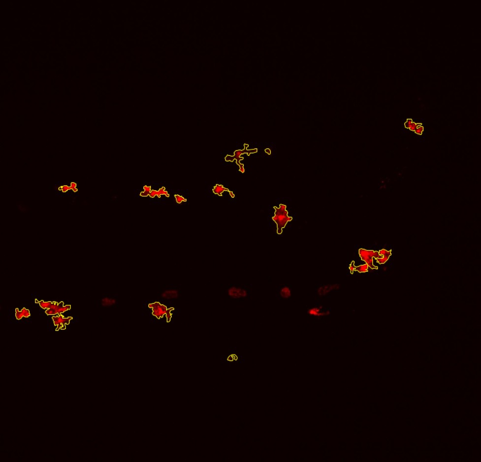
Here is an example of an image that will be placed in the x sets (whether it is the training or the test set) on the left. And on the right, each yellow lining represents a ROI (region of interest). Those are saved in a zip file and in the y sets.

Note
Documentation on Fiji can be found here.
Next, the kartezio package that will help us build the model needs two other files: META.json and dataset.csv.
The META file is here to help the package recognize the formats of the different objects in the dataset folder.
import json

# Path to the JSON file
meta_path = "model/dataset/META.json"

# Content of the JSON file
meta_data = {
    "name": "Macrophage",
    "scale": 1.0,
    "label_name": "macrophage",
    "mode": "dataframe",
    "input": {"type": "image", "format": "hsv"},
    "label": {"type": "roi", "format": "polygon"},
}

# Create the JSON file with the content in it
with open(meta_path, "w", encoding="utf-8") as f:
    json.dump(meta_data, f, indent=4)

print(f"File {meta_path} created successfully!")
The CSV file is here to help kartezio read your dataset.
from Set_up.dataset_csv import create_dataset_csv

create_dataset_csv(input_folder="model/dataset", output_csv="model/dataset/dataset.csv")
Your two files are now created and located in the model/dataset folder. We can now train our model.
Training
Now that we have the structure kartezio needs to function correctly, we can create and train a model using the create_segmentation_model function of the kartezio package. You can find the following code in the Set_up/train_model.py file.
from kartezio.apps.segmentation import create_segmentation_model
from kartezio.endpoint import EndpointThreshold
from kartezio.dataset import read_dataset
from kartezio.training import train_model

import time
from datetime import timedelta

t0_train = time.time()

DATASET = "model/dataset"
OUTPUT = "model/models"

generations = 1000
_lambda = 5
frequency = 5
rate = 0.1
print(rate)
model = create_segmentation_model(
    generations,
    _lambda,
    inputs=3,
    nodes=30,
    node_mutation_rate=rate,
    output_mutation_rate=rate,
    outputs=1,
    fitness="IOU",
    endpoint=EndpointThreshold(threshold=4),
)

dataset = read_dataset(DATASET)
elite, a = train_model(model, dataset, OUTPUT, callback_frequency=frequency)

t1_train = time.time()
elapsed_train = int(t1_train - t0_train)
Testing
Now that you trained your model, you can test it to see if it gives good predictions.
import numpy as np
import pandas as pd

from kartezio.easy import print_stats
from kartezio.dataset import read_dataset
from kartezio.fitness import FitnessIOU
from kartezio.inference import ModelPool

t0_test = time.time()

scores_all = {}
pool = ModelPool(f"model/models", FitnessIOU(), regex="*/elite.json").to_ensemble()
dataset = read_dataset(f"model/dataset", counting=True)
annotations_test = 0
annotations_training = 0
roi_pixel_areas = []
for y_true in dataset.train_y:
    n_annotations = y_true[1]
    annotations_training += n_annotations
for y_true in dataset.test_y:
    annotations = y_true[0]
    n_annotations = y_true[1]
    annotations_test += n_annotations
    for i in range(1, n_annotations + 1):
        roi_pixel_areas.append(np.count_nonzero(annotations[annotations == i]))
print(f"Total annotations for training set: {annotations_training}")
print(f"Total annotations for test set: {annotations_test}")
print(f"Mean pixel area for test set: {np.mean(roi_pixel_areas)}")

scores_test = []
scores_training = []
for i, model in enumerate(pool.models):
    # Test set
    _, fitness, _ = model.eval(dataset, subset="test")
    scores_test.append(1.0 - fitness)

    # Training set
    _, fitness, _ = model.eval(dataset, subset="train")
    scores_training.append(1.0 - fitness)

t1_test = time.time()
elapsed_test = int(t1_test - t0_test)
elapsed_total = elapsed_train + elapsed_test

print(scores_training)
print(scores_test)

scores_all[f"training"] = scores_training
scores_all[f"test"] = scores_test

pd.DataFrame(scores_all).to_csv("model/scores.csv", index=False)

print(f"Total runtime : {timedelta(seconds=elapsed_total)}")
print(f"Training time : {timedelta(seconds=elapsed_train)}")
print(f"Testing time : {timedelta(seconds=elapsed_test)}")
Model summary
You can get a summary of your model by running the following.
from Set_up.explain_model import summary_model

summaries = summary_model("model")
You can create a csv file for the nodes that will help you understand your model.
for summary in summaries:
    print(summary.to_csv())
You can also access other parameters that are not displayed in the summary, for instance:
print(summaries[0].keys())
And you can extract any object from that list.
print(summaries[0].endpoint)
Model visualization
You can visualize the model you’ve just created and tested by running the following code.
from mactrack.visualisation.viz_model import comp_model

comp_model("./model", train=False)
You have two options to visualize your model:
If you put train=False, it will compare the test set with the predictions on the test set.
If you put train=True, it will compare the training set with the predictions on the training set.
You can then find the results in the output folder.
comp_model("./model", train=True)
Calculate IOU
You have to be careful with the second argument. If you’ve put train=False (default), you will have to use the test set. If you’ve put train=True, you will have to use the training set, which means that your second argument will be ./model/dataset/train/train_y/ and not ./model/dataset/test/test_y/.
from mactrack.visualisation.iou import mean_global_iou

mean_global_iou(
    "./model_output/test_def/ROIs_pred_def/",
    "./model/dataset/test/test_y/",
    "./model_output/comparison/",
)